NGO Another Way
(Stichting Bakens Verzet), 1018 AM
SELF-FINANCING,
ECOLOGICAL, SUSTAINABLE, LOCAL INTEGRATED DEVELOPMENT PROJECTS FOR THE WORLD’S
POOR
|
FREE
E-COURSE FOR DIPLOMA IN INTEGRATED DEVELOPMENT |
|||||
Edition 05: 08 August, 2011.
Edition 07 : 09 February, 2013.
(VERSION EN FRANÇAIS PAS DISPONIBLE)
Information on monetary reform :
NEW Capital is debt.
NEW Comments on the IMF (Benes and Kumhof) paper “The
Chicago Plan Revisited”.
DNA of the debt-based economy.
General summary of all papers published.(Revised edition).
How to create stable financial systems in four
complementary steps. (Revised edition).
How to introduce an e-money financed virtual minimum wage
system in New Zealand. (Revised edition) .
How
to introduce a guaranteed minimum income in New Zealand. (Revised edition).
Interest-bearing debt system and its economic impacts.
(Revised edition).
Manifesto of 95 principles of the debt-based economy.
The Manning plan for permanent debt reduction in the national economy.
Missing links between growth, saving, deposits and
GDP.
Savings Myth. (Revised edition).
Unified text of the manifesto of the debt-based
economy.
Using a foreign transactions surcharge (FTS) to manage the
exchange rate.
(The
following items have not been revised. They show the historic development of
the work. )
Financial system mechanics explained for the first time. “The Ripple
Starts Here.”
Short summary of the paper The Ripple Starts Here.
Financial system mechanics: Power-point presentation.
THE RIPPLE STARTS HERE
1694-2009:
Finishing the Past
By:
manning@kapiti.co.nz 19B
Version
4 18/05/09
Key
words: Debt, Debt model, Economic
theory, Financial System, Fisher equation, Friedman, Inflation, Irving Fisher,
Keynes, Keynesianism, Macroeconomics, Macroeconomic model, Mechanics of debt,
Monetarism, Savings, Economic growth,
SYNOPSIS
This
paper offers a definitive statement of economic activity to replace
Keynesianism and Monetarism. It shows why both the main economic theories of the twentieth
century have failed and what to do about the world financial situation. The
work amends the Fisher equation of exchange (MV=PQ) to allow for structural
changes in the financial system that took place after the Bank of England was
set up in 1694. An economic debt “model”
demonstrates the underlying mechanics of private debt-based banking and the
relationship between the productive and investment sectors. The “model” is
definitive in that it describes actual economic activity. It is used to provide
an historical profile of the
INTRODUCTION
There has long been a
substantial theoretical disconnect between financial and monetary policy and
economic behaviour in the real world.
Recent world events show how limited economists’ understanding of the
mechanisms underlying the monetary policy has been and still is. The basic
mechanisms at the heart of the “modern” financial system itself have never
successfully been put into a logical framework that is robust enough to allow
the underlying relationships to be quantified.
One effort to do so was
provided by Irving Fisher in 1911[1] in his well-known
equation of exchange that takes the form:
MV = PQ (1)
or M= PQ/V (2)
Where: M = the amount of money in circulation
V = the speed of circulation of that money; the
number of times M is used over a given period T
P = the
price level of goods and services an economy produces during time T
Q= the
monetised quantity of goods and services an economy produces during time T.
The product PQ is
what is known today as Gross Domestic Product or GDP. At first sight, the
Fisher equation seems to be self-evident. People have to be able to produce and
exchange goods and services. To the
extent money is used to do this, the total produced must bear a relationship to
the amount of money and the frequency with which it is used.
Verifying the
Fisher equation of exchange, until now, has been difficult. A few people have
tried to do it[2]. The main difficulties have been to work out
reliable estimates for the variables. Historically, only the price level P has
been known within a reasonable margin of error, despite the fantastic work done
by researchers around the world[3].
The relationship presented
here began with an attempt to address a psychological question. “Has peoples’ hoarding behaviour changed over
time?” The question is crucial to
understanding the Fisher relationship.
For a given quantity of goods and services Q, does the price P change
when the amount of money M changes, or does the speed of circulation of that
money, V, change? Or do P and V both
change?
The crude estimate
of V in
The speed of
circulation, V, appears to have been reasonably constant[7] because it essentially represents a
hoarding function. At any given time, most money was “saved”. It can be
surmised that V is a structural rather than a dynamic component in the Fisher
relationship. The immediate response to a change in the money supply M will be
a change on the production side of the equation PQ. If the change in M is rapid, the response
will be a change in prices P until production and demand adjust to compensate
for the change in the money supply. That’s different from what happens with
fresh produce in the supermarket after bad weather. In that case the money side of the equation
remains unchanged and prices rise because production falls. That happens in the
shops regularly and from season to season.
The speed of
circulation on the other hand appears to require a change in people’s behaviour
toward money, or changes in the way the financial system works.
THE BANK OF
Changes in the
economy began with structural changes in the money supply M made possible
through the creation of new money as debt. When the Bank of England was
established in 1694, the money supply, for the first time, became relatively
independent of the supply of gold and silver.
When a bank issues
a new loan, the loan amount becomes an asset in the accounts of the bank. From
the bank’s point of view it’s an asset because the borrower has to repay his
debt to the bank. The new loan asset is offset by an equal liability for the
bank in the form of a money deposit. Money has been created “out of nothing” by
way of a bookkeeping entry. Of course, the loan has to be repaid over
time. As it is repaid, the outstanding
loan is reduced. Once the loan is fully repaid there is no loan remaining and
no residual deposit. The loan and the new money have both been cancelled out of
existence.
The bank gets
nothing from the process itself. As long
as the loan and deposit remain the same there is no profit to the bank and no
way for the bankers to become rich.
Instead, the Bank of England shareholders became rich because they
charged interest on their loans.
Interest has been
paid on loans ever since the use of money became widespread thousands of years
ago. People would loan their hoarded savings to someone else and expect their
savings to increase by the amount of interest they received. The borrowers would usually borrow in the
expectation that doing so would increase their productivity or their fortune in
some other way. For example, buying an ox or workhorse might dramatically
increase production from a farmer’s land. The increased production created by
using the ox or the workhorse would more than offset the interest on the
loan. Both parties were better off as a
result of the investment made by using the borrowed money.
The operative word in all this
is “investment”, the use of money to increase production. The problem with the Bank of England in 1694
was twofold. First, the loans it made to
the government were not to increase production but to help pay the war debts of
the crown. Secondly the Ways and Means Act[8] that authorised the
Bank of England provided for a perpetual fund of interest charged on ships’
“tunnage” and liquor duties. Not only
was the loan for current spending instead of investment, it would never be
repaid. The interest would have to be
funded from taxes forever. Since then,
governments have found it very easy to borrow perpetual debt in this way and
its use has increased steadily over time.
STRUCTURAL CHANGES
IN THE SPEED OF CIRCULATION V
Establishing banks
that create money, the so-called banks of issue like the Bank of England,
structurally altered the financial system by providing a mechanism for the
speed of circulation, V, to change over time.
That mechanism allowed the creation of a
non-productive pool of “unearned”
interest income from deposits.
Unearned income from
deposit interest is a structural part of the debt system. It has nothing at all
to do with production and accumulates solely because new money is created as an
interest-bearing debt. It forms the
basis of the investment sector as distinct from earned savings. The investment
sector is characterised by trading and speculative investment in existing
wealth rather than creating new production and new wealth. Other things being
equal, prices for that existing wealth keep rising because the pool of unearned
income grows as more and more interest is added to it[9].
The banking sector
relies for increased profits on the total money supply M increasing as fast as
possible, thereby allowing the pool of unearned interest to grow quickly.
That’s the main reason the money supply has expanded so quickly. Profit
arising from the bank spread or margin, the difference between the interest
borrowers pay on their loans and the interest banks pay depositors on their
deposits, is a direct function of the money supply M and is, most people would
be surprised to know, largely independent of interest rates. When M goes up bank profits rise. Bank
profits fluctuate with interest rates only when, as a result of perceived
lending risk, they alter their spread, the difference between the interest they
charge on loans and the interest they pay their depositors; or with changes in
the number and size of defaults by borrowers. Such banking activity is part of
the productive sector, but the unearned interest paid by banks on bank deposits
is not.
There is an
inherent conflict of interest between the debt-based banking system and the
productive sector. Capitalism is fundamentally profit-seeking. Banks seek to
increase M to get the greatest profit, while the productive sector receives a
decreasing share of wealth because unearned income shifts money away from the
productive sector to the investment sector. In aggregate, over time, this
drives up asset prices, creating the all too familiar investment bubbles and an
overemphasis on capital gains. Prices
are likely to increase until the point is reached where the expectations of the
investment sector overwhelm the productive economy. This paper will show that
the divergence between capital gains and productive incomes has been increasing
exponentially, guaranteeing future economic collapse unless the financial
system itself is adapted to take account of the mechanics of interest-bearing
debt.
AMENDING THE FISHER EQUATION OF EXCHANGE
The foregoing
discussion suggests the money supply M in the Fisher equation of exchange can
be conceptually divided into two parts.
Money used for production could be called Mp and the unearned income
interest component of M could be called Ms so the Fisher equation can be
written as.
M= Mp+Ms (3)
Mp*Vp = PQ (4)
M = PQ/Vp +Ms (5)
PQ = (M-Ms)*Vp (6)
Mp=M-Ms (7)
Where Mp is the money used for
production,
M is the total money supply,
Ms is the accumulated unearned
income from interest on bank deposits,
Vp is the speed of circulation
of Mp,
P is the price level,
Q is total output of goods and
services.
The unearned income
Ms circulates outside the production cycle so it has no impact on PQ. Hoarding in
times gone by did not structurally increase the money supply M, but the
continual addition of interest on all interest-bearing debt to Ms produces a
structural change in the money supply M and hence, in the original Fisher
equation (Mp+Ms)V=PQ, a structural change in V. That structural change in V has
nothing to do with changes in human hoarding behaviour. It is a mechanical
feature of the interest-bearing debt system.
That may be why so many people have had so much difficulty working with
the Fisher equation of exchange in the past.
In the interest-bearing debt system, all the loans
included in M can never be repaid. The productive money supply Mp from which
they must be repaid is necessarily less than M because M=Mp+Ms. The debt
supporting the unearned income Ms remains forever a burden on the productive
sector.
In equation (4)
Mp*Vp = PQ, if Mp, the productive part of the money supply, is not to actually
shrink, either the total money supply M =(Mp+Ms) must grow by at least the
amount added to Ms, or else the speed of circulation, Vp, of Mp must rise. If
Vp is reasonably constant, as is suspected, then the money supply M must grow
faster than Ms if PQ is to grow.
Since the amount added to M as unearned income from
deposit interest Ms is a percentage of M, the financial system is locked into
exponential growth at least equal to the interest rate on the unearned deposits. The only way to reduce that exponential
growth of M is to reduce or eliminate the interest rate on deposits.
Conceptually, the
effect of unearned interest on deposits is to transfer claims on the real
wealth of the nation from those who produce the economic output PQ to those in
the investment sector who produce nothing.
Houses and other assets become more expensive in terms of the inflated
prices in the investment sector but must be bought using the less inflated
money of the productive sector.
Unless inflation in
the investment sector and the productive sector are equalised, there must be an
ever-widening gap between debt-bound wage and salary earners on the one hand
and the participants in the investment sector with net deposits in the banking
system on the other hand. At the moment
there is a kind of dual exchange rate operating in favour of investors. Wage
and salary earners have to use the less inflated money they earn to buy assets
“priced” in the inflated dollars of the investment sector.
The original Fisher
equation took no account of the investment sector unearned income Ms. Nor did
it take into account offshore borrowings. Countries owing money offshore have
to pay interest on those offshore loans even though the corresponding money
(foreign debt) does not appear in any domestic bank account.
Interest on the accumulated
foreign debt, like interest on the domestic debt, has to be funded from the
productive economy. Unearned interest payments being made on foreign accounts
have to be included in unearned income Ms if it is to truly represent the whole
of the investment pool of unearned income, as well as the interest on domestic
accounts. The domestic money supply is no longer the sole “base” of the “money”
supply as it used to be. Distortions caused by omission of foreign debt would
have been minor for most countries in the early twentieth century when Fisher
first proposed his equation of exchange. They are often more significant today
because some countries like New Zealand have very large current account
(foreign) debts while others like Japan have large current account (foreign)
surpluses.
DEBT
IS MONEY
Until the Bank of
England was established in 1694 virtually all money in circulation was coin.
From 1694 until perhaps the middle of the nineteenth century much of the money
in circulation was made up of bank notes and coins. That changed through the 19th
century. For example, in
By July 2008, 99%
of the
If debt
is money, the variables in equation 7 can be restated:
Debt for production Mp=
(Total
Debt)
With this in mind,
the original Fisher equation can be further reformulated so the speed of
circulation V becomes a function of the productive debt Mp only. This will be
called Vp. The justification for this is that unearned income derived from Ms
produces nothing, though it remains a valuable measure of the concentration of
wealth in the economy.
Since the Total
Debt Md= debt for production Mp + debt supporting unearned income Ms, (equation
3) and Mp=Md-Ms, (equation 7) the newly revised form of the Fisher equation (5)
using just the speed of circulation Vp of the productive debt Mp becomes:
M(d)=PQ(d)/Vp +Ms (8)
Where:
Mp= debt used for production
Vp = speed of circulation of
debt used for production
M(d) = total debt
Ms= debt held by productive
sector to fund unearned income on the total debt,
P = prices
Q(d) = quantity or output of production produced
by Mp
PQ(d) does not include any contribution to a
nation’s GDP resulting from cash transactions.
The three main
components of the total debt Md are the domestic debt, the foreign debt and
central bank reserves. In this work the domestic debt is taken to be the
Domestic Credit while the foreign debt is taken to be Accumulation of all the
Current Account deficits over time. The
reserves, R, held by the central bank, must be subtracted when calculating Md
because they represent debt included in Domestic Credit that is not in
circulation[11]. R is small
compared with
A national current account
deficit really means a country is consuming production created by money
circulating abroad instead of using local money to generate the whole of its
economic product locally. From the point of view of the new Fisher equation
(8), debt circulating in a foreign country is no different from debt
circulating locally. Likewise, the interest being paid on offshore borrowing is
unearned income and its corresponding debt forms part of Ms in the revised
version of the Fisher equation (8) described above. It is conceptually no
different from other unearned income supported by Ms.
When considering
the new Fisher equation in the context of the modern economy the total debt Md
in equation (8) Md=PQ(d)/Vp+Ms has to
include the foreign debt and the debt Ms arising unearned income has to allow
for the interest paid on foreign debt as well as the deposit interest paid on
domestic debt.
The accumulated
national current account debt will be called Dca and the domestic credit
component will be called Ddc. Central bank reserves will be called R. These are
the three main components of total debt
There is one
further variable to be considered. It is the debt, to be called Mv in this
work, directly borrowed to support speculative investment. It belongs with Ms in the investment sector
and is likely to be associated with rapid expansion of debt during an
investment boom.
Mv is, literally, the investment“bubble” that inflates
with booms and decays with busts. The revised Fisher relationship enables it to
be identified and quantified.
Mv appears to have
been especially prominent in the “wild west” days in New Zealand during the mid
1980’s, during the dotcom boom in the late 1990’s and apparently from 2005 to
2009 when there was a substantial new debt bubble. Mv has almost certainly
played a significant role in the
The revised Fisher
equation (8) can be rewritten as:
Md= (Ddc+Dca-R) = PQ(d)/Vp +
(Ms+Mv) (9)
Or, since from equation (7)
Mp= (Md-Ms),
Mp = (Ddc+Dca-R) –(Ms+Mv) (10)
where:
Dca = accumulated current account debt,
Ddc = domestic credit,
R = central bank reserves[12],
Vp = speed of circulation of
debt used for production,
Md = total debt,
Ms = debt held by productive sector to fund the unearned
income on the total debt,
Mv = debt borrowed for speculative investment rather than production
P = prices,
Q(d) = quantity of production produced by debt Mp,
Mp = debt used for production
= (Md-Ms).
The debt that
supplies the investment pool Ms is always “owned” by the productive sector, not
the investment sector. It is a structural part of the total debt Md but its
monetary equivalent in the form of unearned income resides outside of and is
separate from the productive sector. In bad times when there are “losses” in
the investment
sector, the debt Ms remains numerically intact whatever happens in the
productive economy. It is theoretically unrepayable unless debt-free money is
introduced into the financial system or unless there is a negative deposit
interest rate. Actual investment sector losses (write downs) must come either
from the investment sector debt Mv or from the productive sector funding Mp,
reducing the financial system liquidity as was apparent in the
When investors lose
their shirts, their unearned income deposits (their share of deposits arising
from Ms) are merely shifted to someone else. They are still unearned income
deposits. At the end of the day, were
all of the investment sector debt Mv and the productive sector funding Mp to be
eliminated, people in the productive sector would still be left with the debt
Ms. Another, presumably different, group would hold all of the corresponding
unearned income deposits. That is a conceptual endpoint of the present
financial system. Hunger, despair, riots
and even revolution would presumably lead to a change in the financial system
long before such a conceptual endpoint is reached.
AN
ECONOMIC REVOLUTION FROM THE NEW FISHER EQUATION
Take the revised form of the
Fisher equation of exchange:
Md= (Ddc+Dca-R) = PQ(d)/Vp +
(Ms+Mv) (9)
Mp = (Ddc+Dca-R) –(Ms+Mv) (10)
In each production
cycle part of Mp arises from the creation of new debt in the production
phase. In general that new debt is
subsequently cancelled in the consumption phase. There are literally millions
of these cycles continuously superimposed one on the other.
This leads to a
startling conclusion that reflects the beauty of devising a debt model of the
economy. In aggregate, the speed of circulation Vp of the productive debt Mp
must theoretically be 1 when used in the new form (9) of the Fisher equation of
exchange[13]. Each tranche of
new debt Mp is notionally repaid as its product PQ(d) is consumed. Each tranche
of debt is used just once. It is impossible to spend the money arising from a
loan more than once. To spend more means
borrowing more. The shortfall, amounting to the unearned interest income
transferred to Ms in each production cycle, has to be borrowed in addition to
the tranche needed to fund the next production cycle. Much, if not most, of
increased productivity in the productive sector is immediately “lost” to the
investment sector.
The debt Mp in the productive economy must grow if the
economy is to grow. That is the fundamental source of the exponential growth
imperative in all modern debt based economies.
Equations (9)
and (10) are debt based. If Vp in equation (9) is 1, it follows that
the speed of circulation of the monetary equivalent of Mp must also be 1 if
equation (9) is to hold when expressed in monetary terms. That the monetary
“footprint” of Mp can be used only once in generating the nation’s GDP at first
appears to be surprising, remembering that the historical value of the speed of
circulation V in the original Fisher equation in England appears to have been
something like 2.5[14]. Conceptually, each production cycle is
separate. The debt for production is
borrowed and the corresponding money is first used and then repaid as goods and
services are production and consumed.
The money is re-borrowed and repaid again during the next cycle. In aggregate, intermediate productive
transactions are a “pass the parcel” exercise, accumulating and retiring debt
through the production and consumption process.
Table1[15] shows an
indicative model for the
Md= (Ddc+Dca-R) = PQ(d)/Vp +
(Ms+Mv) (9)
It solves the
equation for the speed of circulation in the productive economy, Vp, by
restating equation (9) as:
Vp = PQ(d)/[(Ddc+Dca-R)-(Ms+Mv] (11)
Figure 1 shows the
speed of circulation Vp of the productive debt Mp used to generate the debt
derived portion of
In
Despite the evident
data limitations Table 1 is believed to give a reasonable first approximation
of the application in New Zealand of the revised Fisher equation Vp = PQ(d)/[(Ddc+Dca-R)-(Ms+Mv] (11).
The new version of
the Fisher equation of exchange (9) can be applied at any point in time, in
principle providing macro economic data in real time if the debt and interest
rate numbers are available.
Were interest on
bank deposits to be reduced to zero, the pool of unearned income Ms would
remain constant at its present level.
With the speed of circulation Vp=1, the increase in GDP would become a
direct function of the Total Debt Md-Mv.
The effect of
applying the modified Fisher equation (11) Vp =
PQ(d)/[(Ddc+Dca-R)-(Ms+Mv)] in
the modern economy can be stated as follows:
In a cash-free debt
based economy with zero interest rates on deposits the increase in GDP (PQ)
equals the increase in the total debt Md less any change in direct speculative
investment Mv.
In
the debt system, economics is primarily a matter of debt management.
TABLE 1 MODIFIED FISHER
APPLICATION NEW ZEALAND 1978-2008
USING AGGREGATE FIGURES
|
1 |
2 |
3 |
4 |
5 |
6 |
7 |
8 |
9 |
10 |
11 |
12 |
13 |
|
Year |
CA* |
DC* |
I%* |
GDP* |
Mo |
Vo |
PQd* |
Md* |
%Md* |
Ms |
Vp’ |
Mv* |
|
1978 |
4.8 |
9(Est) |
8.7 |
15.3+ |
0.404 |
19 |
7.6 |
13.6 |
36 |
4.75 |
0.86 |
1.21 |
|
1979 |
5.3 |
9.8 |
7.0 |
17.4+ |
0.455 |
19 |
8.8 |
14.9 |
36 |
5.11 |
0.90 |
1.01 |
|
1980 |
6.1 |
11.2 |
8.0 |
20.3+ |
0.491 |
19 |
11.0 |
17.1 |
36 |
5.57 |
0.95 |
0.52 |
|
1981 |
7.0 |
12.9 |
9.0 |
23.6+ |
0.535 |
19 |
13.4 |
19.6 |
36 |
6.16 |
1.00 |
0.08 |
|
1982 |
8.6 |
15.9 |
9.0 |
28.7+ |
0.593 |
19 |
17.4 |
24.2 |
36 |
6.87 |
1.00 |
-0.07 |
|
1983 |
10.5 |
21.8 |
8.8 |
32.3+ |
0.650 |
19 |
20.0 |
32.0 |
36 |
7.77 |
0.82 |
4.31 |
|
1984 |
12.4 |
25.4 |
10.1 |
36.0+ |
0.652 |
19 |
23.6 |
37.5 |
36 |
9.03 |
0.83 |
4.88 |
|
1985 |
15.7 |
30.4 |
10.5 |
40.7+ |
0.718 |
18 |
27.8 |
45.8 |
36 |
10.60 |
0.79 |
7.43 |
|
1986 |
19.7 |
40.0 |
14.3 |
46.9+ |
0.831 |
17 |
32.8 |
59.4 |
36 |
13.31 |
0.71 |
13.31 |
|
1987 |
22.5 |
44.6 |
14.2 |
55.3+ |
0.868 |
17 |
40.5 |
66.8 |
36 |
16.54 |
0.81 |
9.71 |
|
1988 |
24.9 |
51.8 |
12.3 |
63.2+ |
0.861 |
17 |
48.6 |
76.4 |
42 |
20.24 |
0.86 |
7.58 |
|
1989 |
25.5 |
53.2 |
11.5 |
67.9+ |
0.953 |
17 |
51.7 |
78.3 |
53 |
24.95 |
0.97 |
1.70 |
|
1990 |
28.3 |
58.3 |
10.8 |
71.5+ |
1.075 |
17 |
53.2 |
86.2 |
64 |
30.84 |
0.96 |
2.38 |
|
1991 |
30.2 |
63.1 |
10.8 |
73.3+ |
1.120 |
17 |
54.3 |
92.9 |
67 |
37.12 |
0.97 |
1.55 |
|
1992 |
32.1 |
68.9 |
8.4 |
72.9+ |
1.024 |
17 |
55.5 |
100.6 |
70 |
42.81 |
0.96 |
2.32 |
|
1993 |
34.0 |
70.9 |
6.3 |
76.1+ |
1.082 |
16.8 |
58.0 |
104.5 |
72 |
47.46 |
1.02 |
-1.21 |
|
1994 |
35.9 |
77.9 |
5.4 |
80.9+ |
1.219 |
16.5 |
60.8 |
113.4 |
74 |
51.82 |
0.99 |
0.8 |
|
1995 |
40.0 |
82.5 |
5.8 |
86.3+ |
1.301 |
16
|
65.5 |
122.0 |
76 |
57.01 |
1.01 |
-1.14 |
|
1996 |
45.1 |
91.9 |
7.2 |
93.2 |
1.399 |
15.5 |
71.5 |
136.5 |
78 |
64.27 |
0.99 |
0.83 |
|
1997 |
51.0 |
102.0 |
7.3 |
98.0 |
1.503 |
15 |
75.5 |
152.5 |
80 |
72.70 |
0.95 |
5.04 |
|
1998 |
56.5 |
112.2 |
6.5 |
101.7 |
1.547 |
14.5 |
79.3 |
168.2 |
82 |
81.25 |
0.91 |
7.71 |
|
1999 |
60.9 |
122.5 |
6.4 |
103.4 |
1.682 |
11 |
84.9 |
182.9 |
84 |
90.69 |
0.92 |
8.51 |
|
2000 |
68.0 |
134.6 |
4.4 |
109.1 |
1.830 |
9 |
92.6 |
202.1 |
86 |
97.97 |
0.89 |
11.37 |
|
2001 |
73.2 |
143.9 |
5.4 |
116.0 |
2.044 |
7 |
101.7 |
216.5 |
88 |
107.9 |
0.94 |
6.86 |
|
2002 |
76.6 |
159.6 |
4.7 |
124.1 |
2.237 |
5 |
112.9 |
235.7 |
90 |
117.5 |
0.96 |
5.17 |
|
2003 |
81.6 |
170.6 |
4.6 |
131.0 |
2.289 |
3.5 |
123.0 |
251.6 |
92 |
127.8 |
0.99 |
0.76 |
|
2004 |
87.9 |
184.5 |
4.4 |
139.8 |
2.483 |
2.75 |
133.0 |
271.8 |
94 |
138.6 |
1.00 |
0.13 |
|
2005 |
98.2 |
209.9 |
4.8 |
149.1 |
2.686 |
2 |
143.7 |
306.5 |
95 |
151.8 |
0.93 |
10.84 |
|
2006 |
112.7 |
223.8 |
5.7 |
156.6 |
2.811 |
1.5 |
152.4 |
334.7 |
96 |
169.3 |
0.92 |
12.86 |
|
2007 |
126.4 |
249.7 |
6.2 |
165.1 |
2.945 |
1.0 |
162.2 |
374.5 |
97 |
190.6 |
0.88 |
21.34 |
|
2008 |
140.2 |
273.3 |
7.0 |
177.6 |
3.038 |
0.5 |
176.1 |
411.6 |
98 |
217.6 |
0.91 |
17.80 |
|
2009 |
155 |
292.9 |
6.49 |
183 |
3.44 |
0 |
183.0 |
444.1 |
99 |
245.9 |
0.92 |
15.93 |
CA = accumulated current
account deficit NZ$b; DC=Domestic Credit
NZ$b; I%= annual average deposit interest rate;
GDP = Official SNA GDP NZ$b; PQd=Column 5- Column 6 x column 7
NZ$b; Md=Column2 +Column3-RBNZ “capital
reserves” NZ$b, %Md = estimated
proportion of Md funded at deposit interest rate; Ms =Column 9 *x Column 10 x Column 4 accumulated NZ$b; Vp’=(Column 9-Column
11)/Column 8NZ$b; Mv =Column 9- Column 5-Column 11 NZ$b + GDP figures based on SNA 68.
Were Ms and Mv zero in the
revised Fisher equation (11), it would
essentially be returned to the form of the original Fisher equation (1) MV=PQ except that the debt-derived equivalent
of M in the original equation is now expressed as (Ddc+Dca-R).
At the time Fisher first
proposed the Fisher equation of exchange in 1911, most economic transactions
were still cash transactions[19].
That is not to suggest
for a moment there is no role for economic and monetary policy. The allocation
of available human and natural resources and distribution of wealth are
immensely important issues in modern societies.
But there is no alchemy of economics and never was, any more than was
the case in late medieval
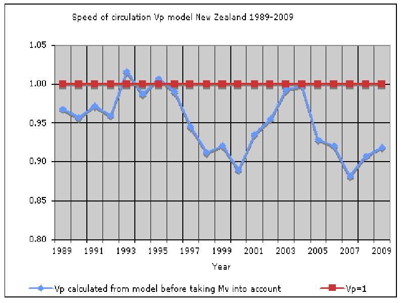
Figure 1 shows Vp
plotted for New Zealand 1989-2009 from Table 1 before taking into account the
speculative investment Mv. Mv is the
debt needed to bring Vp back to 1.
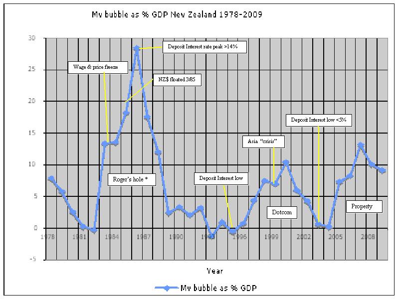
Figure 2 shows the
Mv bubbles as a percentage of GDP that result when Vp is 1. Figure 2 suggests the dotcom bubble at the
turn of the century and the property bubble 2005-2009 were both smaller than
Mv bubbles
dissipate through the repayment (or
write-off) of the speculative debt. Speculative investors sell off assets to
the holders of Ms unearned income deposits or those with earned savings forming
part of
BANKS
AND BANKING
Generally speaking, the larger
the Total
FIGURE 1: SPEED OF CIRCULATION Vp’ OF PRODUCTIVE DEBT
NEW ZEALAND 1989-2009 FROM TABLE 1*
(CLICK HERE FOR FIGURE 1 : THE SPEED OF
CIRCULATION Vp OF PRODUCTIVE DEBT IN NEW ZEALAND 1989-2009 )
Vp’ greater than 1.0 arises
from data and modelling error
FIGURE 2 BUSINESS CYCLE BUBBLES AS PERCENTAGE OF GDP
(CLICK HERE FOR FIGURE 2 : BUSINESS
CYCLE BUBBLES AS PERCENTAGE OF GDP)
* Named after finance minister Douglas. Mv was
substantial through this period of wild speculative expansion though it appears
to have begun earlier. Mv below 0 arises
from data and modelling error income Ms,
the only way to fully repay that new debt is by creating yet more new debt on
which yet more interest has to be paid.
This ongoing process produces the exponential increase in total debt Md,
(and therefore Ms), in the present financial system. Exponential trendlines can be overlaid on the
historical curves for total debt Md, the investment sector Ms and the
accumulated current account deficit Dca (1986-2009) from Table 1[22].
Not only are those
debt trend curves exponential, they show clearly that the investment sector in
New Zealand has been growing exponentially at about 11.2%, substantially faster
than the total debt and current account which have each been growing at about
8.6% and 8.9% respectively. The rapid growth of Ms has very serious monetary
policy implications because it means the productive debt Mp is shrinking as a
proportion of total debt
Monetary policy in
the Western world has evidently and, one would like to hope, inadvertently,
supported this stranglehold by banks over the economy. The only mechanism
presently in use to manage the growth of total debt Md is the interest rate
that in most countries is indirectly controlled by central banks like the US
Federal Reserve. Many of those central banks are themselves powerfully
influenced by the private sector.
Increasing interest
rates to manage inflation has two immediate effects. First, it further
increases the flow of money from the productive sector to the investment sector
by increasing the unearned income pool Ms. Secondly it will tend to increase
bank profits wherever, in response to higher perceived lending risks, the banks
increase their spread or gross interest margin on their loans[23]. Raising the price
of productive debt Mp squeezes demand for it. Jobs are lost. Ordinary people
have less money to spend because more of their income is used to service (pay
interest on) their existing debt. Home ownership becomes difficult if not
impossible. This shift can be called the “transfer effect”.
The transfer effect
is the main reason the use of interest rates to manage the economy has now
failed around the world. In
The revised Fisher equation of exchange proves
conclusively that the use of interest rates for economic management works, if
it works at all, only at extraordinary human cost. The revised Fisher equations
developed in this paper provide a compelling theoretical basis for changing the
world’s financial architecture.
LIQUIDITY
AND CIRCULATING DEBT
The productive debt
Mp is made up of a foreign component Dca, the accumulated current account
deficit, and a domestic component Mcd which is equal to the domestic credit Ddc
less the investment sector debt Ms less the central bank reserves R. Mcd can be
called the “circulating debt”.
Md=Mp+(Ms+Mv) =
(Dca+ Mcd) + (Ms+Mv) = Dca+Ddc -R (12)
Other indicators
can be readily developed using these simple relationships. For example, the “circulating debt” Mcd can be defined as
Mcd= (Mp-Dca) = Ddc-(Ms+Mv)-R (13)
where:
Dca is the
accumulated national current account deficit,
Ddc is the domestic
credit,
Mcd represents the debt
actually available to be used in producing the domestic part of the gross
domestic product produced by debt (PQ(d)),
Mp, Ms, Md. Mv and
R are as previously defined.
The portion of the
gross domestic product produced by domestic debt can be called PQ(dom). It can be defined as:
PQ(dom) =
PQ(d)-PQ(ca) (14)
Where:
PQ (dom) is the
domestic part of QP(d),
PQ(ca) is the
contribution to PQ(d) resulting from the current account,
PQ(d) is as
previously defined.
The speed of
circulation Vcd of the “circulating debt” Mcd
can be defined as :
Vcd =
PQ(dom)/Mcd =
PQ(dom)/(Ddc-(Ms+Mv)-R) (15)
Mcd is the debt
actually available to produce the domestic component PQ(dom) of output PQ(d)
because the foreign debt Dca is committed offshore and is not available for
domestic production. In one sense it is the closest modern equivalent to the
money supply M in the original Fisher equation of exchange MV=PQ (1) and is
believed to be a very sensitive indicator of economic activity. In a world of
instantaneous transaction settlement, most of Mcd represents earned savings
plus transaction account balances.
The speed of
circulation Vcd is believed to be comparable to the speed of circulation V of the
money supply M in the original Fisher equation (1) though it is more virtual
than real. In the interest-bearing debt system the speed of circulation, Vp, of
Mp is 1. Because Dca is unavailable to
the domestic economy except as debt in bank accounts the residual part of Mp,
Mcd, appears to “work harder”. Most of
the earned savings that make up Mp belong to overseas savers when in a healthy
economy those savings would be held in
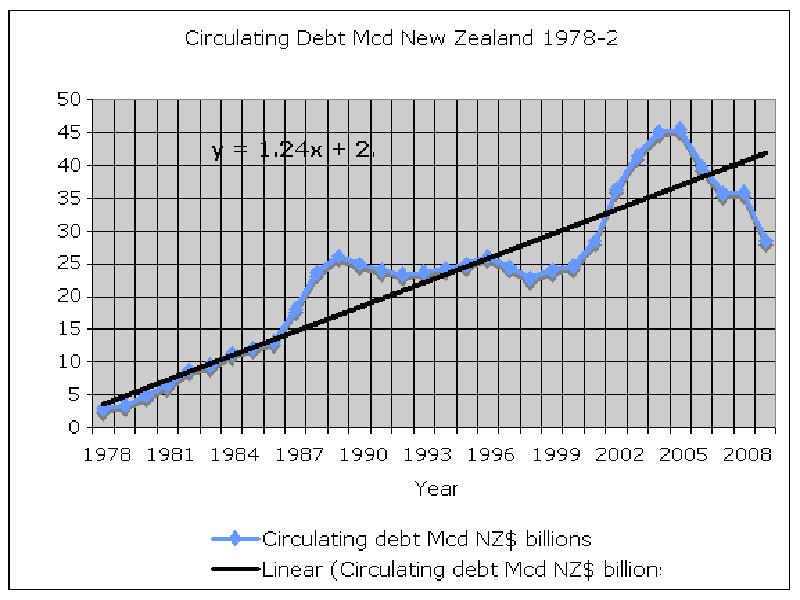
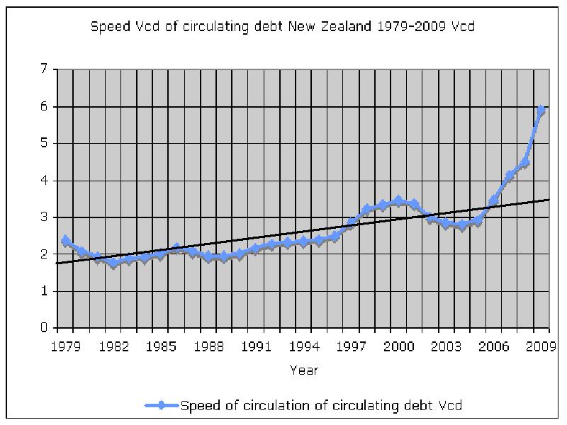
Figures 3 and 4
show Mcd and Vcd for New Zealand, 1979-2009.
They show that the
speed of circulation Vcd increased steadily in
FIGURE 3:
(CLICK HERE FOR FIGURE 3 : CIRCULATING DEBT Mcd IN NEW ZEALAND 1979-2009
)
FIGURE 4: SPEED OF CIRCULATION Vcd OF CIRCULATING DEBT
Mcd NEW ZEALAND 1979-2009[25]
Because of
substantial fluctuation of the circulating debt for production Mcd during
modern business cycles, Vcd is thought to be much less stable now than in past
centuries.
The circulating
debt for production Mcd is thought to be an excellent (inverse) numerical
measure of the liquidity of the financial system.
Figures 3 and 4
show the three boom and bust cycles (mid 1980’s equities, late 1990’s dotcom,
2005-2008 property)
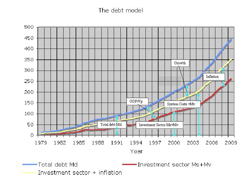
THE
DEBT MODEL
The revised Fisher equation of
exchange Md= (Ddc+Dca-R) = PQ(d)/Vp + (Ms+Mv)
(9)
offers a very simple debt
model of the economy.
It is shown in
Figure 5 where the total debt Md, and unearned income Ms plus speculative
investment Mv, are plotted against time.
PQ(d)/Vp (=Nominal GDP) is the difference between the two curves.
The dependence of
gross domestic product (GDP) on the total
debt Md and the interest rate on bank deposits in the modern cash-free economy
has truly profound implications. The speed of circulation in the productive
sector Vp is fixed at 1. Increases in unearned income arising from Ms depend
directly on the deposit interest rate.
In the light of the
worldwide financial chaos of 2007-2009 the first order debt model shown in
Figure 5 provides a powerful argument in support of public control of a
nation’s financial system. The present
system leaves the world economy at the mercy of privately owned institutions
working for private profit by allowing irresponsible increases of the total
debt, Md and its associated bubble formation.
It isn’t possible
to have a simpler model of the economy than:
Total
debt Md=Nominal GDP (Mp)+Unearned Income Ms + speculative investment Mv.
That is especially
so when, with a simple reconfiguration of the financial architecture, Mv can be eliminated and Ms held constant. That would make the economy
directly dependent on
Total debt, Md, in
New Zealand has grown exponentially by an average of about 8.6% per year since
1986 while the unearned income investment sector as been expanding at the rate
of 11.2% per year. Unless checked, the
only possible outcome for the system over time is for the system liquidity
(Figure 3) to be squeezed toward zero, producing fundamental economic collapse[27].
It is therefore imperative that liquidity be injected
into the system urgently by increasing the domestic credit and largely
eliminating the growth of the investment sector Ms. The model can be used to
quantify the liquidity needed to utilise each nation’s maximum growth capacity.
FIGURE 5: THE DEBT MODEL FOR
THE
(CLICK HERE FOR FIGURE 5 : THE DEBT
MODEL FOR THE NEW ZEALAND ECONOMY )
DEPRESSIONS,
RECESSIONS AND DIFFERENTIAL ANALYSIS
The revised Fisher
equation (9)
Md= (Ddc+Dca-R) =
PQ(d)/Vp + (Ms+Mv)
shows the
relationships among the total debt Md, the total productive output PQ(d), the
speed of circulation of the productive debt Vp, the debt arising from accumulated
unearned income Ms and speculative investment Mv over time. Following basic
differential methods the equation can also be written:
dMd/dt = d/dt (Ddc+Dca-R) = d/dt[PQ(d)/Vp +
(Ms+Mv)] (16)
where over any
small period of time dt, the change in the total debt Md = the change over the
same time dt of PQ(d)/Vp +(Ms+Mv).
There is quite a
lot more variability in the figures calculated this way compared with Table 1
because additional error is introduced by multiple subtractions of large numbers.
Using the
differential approach allows the new debt model to show how the economy is
performing in practice. With better data economic performance could be assessed
monthly, or even, theoretically, in real time.
The differential approach using annual data from Table 1 is shown in
Figure 6. The recorded consumer price
index (CPI) inflation has been added to demonstrate business cycle booms and
busts. Figure 6 is indicative only
pending better model data and calibration.
Of particular
interest in differential equations is what happens at maxima and minima, that
is, at high points and low points.
Referring again to equation (16),
When dMd/dt = 0, d[PQ(d)/Vp+
(Ms+Mv)]/dt = 0, so d/dt PQ(d)/Vp = -d (Ms+Mv)/dt
If there is no
increase in the total debt, nominal economic output PQ(d)/Vp must contract by the amount of unearned income that has to
be transferred to the investment sector and any increase in speculative
investment Mv. For nominal economic output to increase at all, Md must increase
by at least the amount transferred to Ms and invested in Mv. This provides, for the first time, an
absolute definition of a depression, namely when dMd/dt
is less than d(Ms+Mv)/dt.
A depression occurs when the change in the total debt
over time is less than what is needed to service the unearned interest that has
to be paid to the investment sector Ms plus any increase in speculative
investment Mv, that is, when there is no provision for either inflation or
growth.
A similar, absolute,
definition of a recession is when dMd/dt is less than d(Ms+Mv)/dt plus
provision for inflation. Provision for
inflation and unearned income can together be considered financial system
costs. Economic growth occurs only when and to the extent that dMd/dt exceeds
the financial system costs plus speculative investment Mv.
A recession occurs when the change in total debt over
time is less than what is needed to service the financial system costs, being
the unearned interest that has to be paid to the investment sector Ms plus
inflation, plus speculative investment Mv.
The difference
between a recession and a depression is that a recession provides for inflation
but not growth, while a depression provides for neither growth nor inflation.
The model can be
used to provide specific measurable monetary targets to avoid recessions and
depressions. The targets can easily be identified in advance and new debt
injected into the system to maintain growth.
FIGURE 6: INDICATIVE REVISED FISHER DIFFERENTIAL EQUATION
(16) FOR THE
(CLICK HERE FOR FIGURE 6 : NZ
ECONOMY 1979-2009 DIFFERENTIAL METHOD )
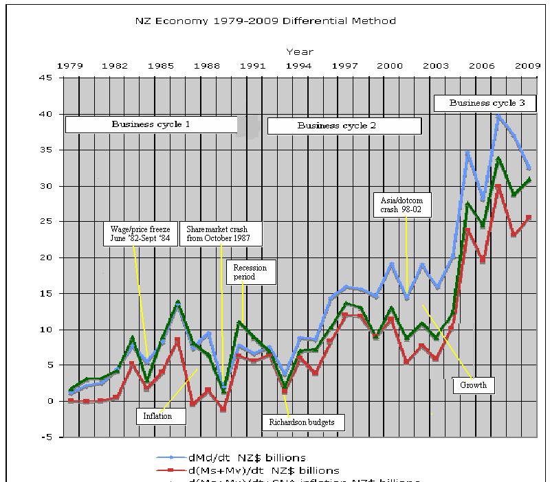
*Preliminary data only; March
years: to show how the model works in
practice.
The chart applies only to
PQ(d) the GDP produced by debt (see equation 16): it does not include GDP
created through the use of cash. The banking sector seized up in 1989 and 1993
much as it did in 2008-2009.
As long as private
interest-bearing debt continues to fund economic activity, it is fundamental
that the total debt dMd/dt continue to expand, no matter what else is happening
in the economy. In the midst of a major
economic downturn in
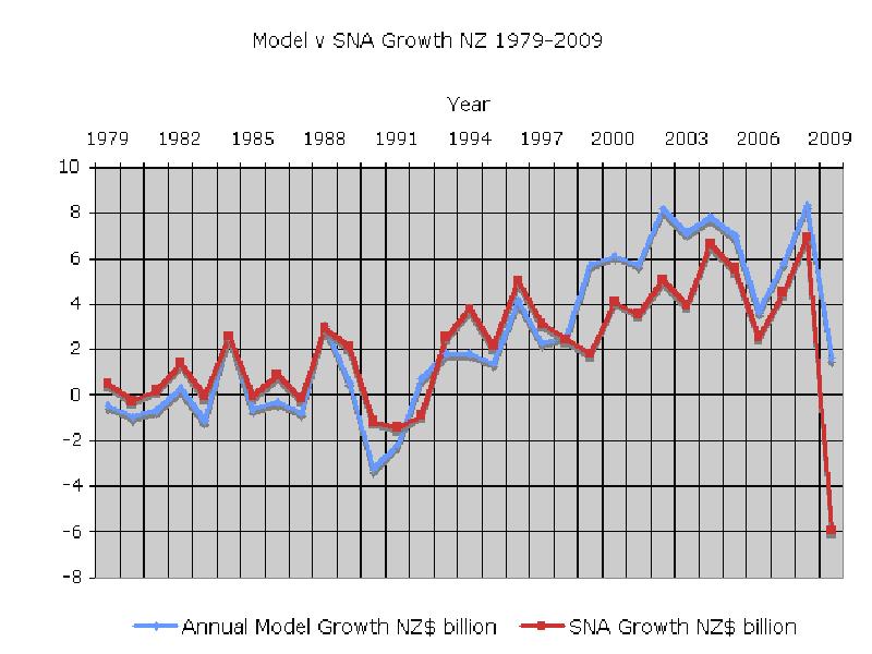
Figure 7 shows the
model growth from Figure 6 plotted against the measured SNA growth from
1979-2009. While Figure 7, like Figure
6, is only preliminary, the model pattern follows the SNA growth trend very
well except for 1999[28]. The model growth figures tend, on the whole,
to be lower than the SNA growth figures because they arise from the use of debt
only. They do not include growth arising from cash transactions during the
period prior to the rapid expansion of EFTPOS beginning in the March 1999
year.
FIGURE 7: MODEL GROWTH COMPARED WITH SNA GROWTH IN THE
(CLICK HERE FOR FIGURE 7 : MODEL v. SNA
GROWTH NZ 1979-2009.)
THE
GENERAL RESTATEMENT OF THE FISHER EQUATION OF EXCHANGE
A general economic model
aligned to the original Fisher equation of exchange is
PQ = (
Where PQ is the GDP,
Md,Ms,Vp,Mv are as described elsewhere
in this paper, (for example equation (9)):
Md is the total debt,
Ms is the debt representing
unearned income on deposits,
Mv is the debt borrowed for
speculative investment rather than production
Vp is the speed of circulation
of Mp (
Mo is the circulating currency
contributing to output,
Vo is the speed of circulation
of Mo,
Eo is circulating electronic
debt-free currency,
Veo is the speed of
circulation of Eo (and must be equal to Vcd).
This general
revision of the original Fisher equation of exchange allows the model to apply
to countries that are not yet cash-free, and countries where debt-free
electronic cash or E-Notes are introduced to replace bank debt.
INFLATION
The debt model
proposed in this paper offers radical new insights into the nature and causes
of inflation.
The revised
differential form of the Fisher relationship:
dMd/dt = d/dt (Ddc+Dca-R) = d/dt[PQ(d)/Vp +
(Ms+Mv)] (16)
includes dMs/dt, the
structural increase of unearned income in the debt system. Conceptually dMs/dt is borrowed into
existence through each production cycle and is passed by way of interest on the
total debt Md through the economy to deposit holders. Ms is unproductive and
represents a structural cost of the debt system. As long as dMs/dt remains the same over time
the same amount of new deposit interest is being passed through the productive
system each cycle. At any point in time, the amount dMs/dt is already included
in the price structure PQ. However, should dMs/dt change over time the amount
included in the price structure PQ must also change. The change over time of
dMs/dt is called the second derivative of Ms. The second derivative of Ms[30] represents systemic inflation in the productive
sector resulting from the debt system because it must be reflected in prices
unless producers accept ever lower margins.
Systemic inflation is inherent in any rise in total debt Md unless the
impact of falling interest rates offsets the impact of rising debt.
Inflation in the
debt system can be divided into three components:
(a) The structural systemic inflation d2Ms/dt, the second derivative of Ms,
representing the changes in dMs/dt over time, and
(b) “PQ”
inflation representing the price-quantity “swap”, effectively the demand curve
of basic economics. PQ inflation happens
when prices rise and the quantity consumed decreases more or less
proportionately. Typical recent examples in
(c) Non-systemic price changes to increase or
maintain margins or profit, such as, for example, to offset wage and salary
increases, tax adjustments and other compliance costs.
PQ inflation does
not change the nominal GDP although it does change the relationship between
inflation and growth within the nominal GDP.
Non-systemic price changes are, like systemic inflation, inflationary.
Aggregate price changes have their counterpart on the income side in increased wages
and salaries, establishing a feedback loop as production costs then continue to
increase[31].
Since Ms, dMs/dt
and d2Ms/dt2 are readily available from Table
The plotted
systemic inflation d2Ms/dt2 figures should always be less
than the CPI figures because they do not include:
(i) “PQ” inflation
(ii) The inflation contribution from increases in
the amount of cash in circulation and used to generate nominal GDP.
(iii) Other non-systemic price changes to
increase or maintain margins or profits.
The contribution
from (ii) is weighted towards the earlier end of the graph in Figure 8 because
Ms was much smaller then and more cash was being used. In
The introduction of
the concept of systemic inflation
leads to a truly radical conclusion;
Raising interest
rates in a cash-free interest-bearing debt-based economy increases systemic CPI
inflation instead of reducing it.
The effect of increasing
interest rates is to starve the productive economy of productive debt as more
of the total debt Md is shifted to Ms, while, at the same time, the demand for
new debt is constrained by the higher interest rates. Under orthodox economic management, systemic
inflation falls after interest rates
begin to fall, that is, after the productive economy has already been slowed or
forced into recession by high interest rates[33]. The rising systemic inflation is
masked, as interest rates are increased, by discounting inventory and by lower
business profitability. To reduce CPI inflation figures when interest rates are
rising, non-systemic inflation must fall faster than systemic inflation rises,
driving the economy into recession.
Since wage and
salary increases often occur in response to price increases they have to be
substantially absorbed by productivity gains or reduced business margins
whenever systemic inflation is similar to measured CPI inflation, as has been
the case during much of the period shown on Figure 8. This raises the possibility that aggregate
productivity gains in the economy could be larger than is generally
acknowledged.
GROWTH AND TRADE
In the revised
Fisher equation (16):
dMd/dt = d/dt (Ddc+Dca-R) = d/dt[PQ(d)/Vp +
(Ms+Mv)]
for the change in
FIGURE 8: MODEL SYSTEMIC INFLATION V CPI INFLATION
NEW ZEALAND 1989-2009
(CLICK HERE FOR FIGURE 8 : MODEL
SYSTEMIC INFLATION v. CPI NEW ZEALAND 1989-2009 )
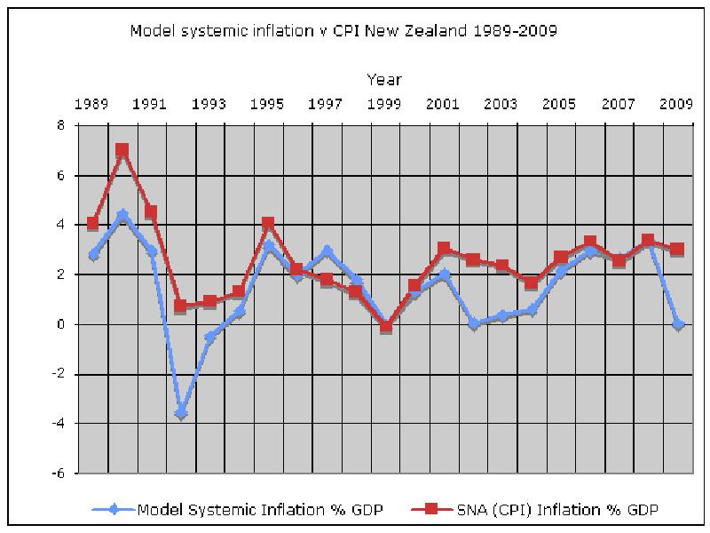
GDP growth in
In terms of the revised Fisher
equations (10) and Figure 5, economic growth in a cash-free debt-based economy
is defined as:
Growth
= Total debt Md – Unearned income Ms- Speculative Investment Mv - Inflation
More importantly,
since from equation (13),
Mcd= (Mp-Dca) = Ddc-(Ms+Mv)-R
Mcd would be up to
NZ$100 billion dollars higher than it is.
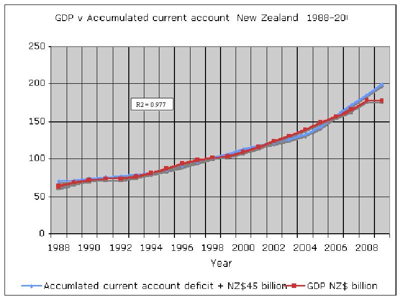
The accumulated
current account deficit Dca is the underlying source of
Had Dca not
accumulated the way it has, there would be no savings problem in New Zealand
even if some of the extra NZ$ 100 billion had been used to retire domestic debt[36]. Any such debt retirement would have meant the
total debt Md and the circulating debt Mcd would each have been reduced by the
same amount. While this would have reduced the GDP[37], new domestic lending would probably
have offset any domestic debt retirement.
FIGURE 9: INCREASE IN GDP v INCREASE IN ACCUMULATED
CURRENT ACCOUNT NEW ZEALAND 1988-2009
(CLICK HERE FOR FIGURE 9 : GDP v.
ACCUMULATED CURRENT ACCOUNT NEW ZEALAND 1988-2009)
Greater savings Mcd
would have been likely to have stimulated more productive investment, expanding
the productive economy. The country’s “wealth” would be NZ$100 billion greater
than it is because the deposits corresponding to the additional debt Ddc would
be held in
The debt model
described in this paper discloses the importance of the current account being
balanced. In practice, the revised Fisher equations show
On the face of it,
Applying the
revised Fisher equation (16) to
dMd/dt = d/dt (Ddc+Dca-R) = d/dt[PQ(d)/Vp +
(Ms+Mv)]
there have been no
bubbles since 1990, so dMv/dt is effectively zero. Deposit rates have also been
practically zero so dMs/dt is also close to zero. R is very small compared with Ddc and Dca and
Vp is 1, leaving, as a first approximation:
dPQ(d)/dt [
Table 2 gives the
key current account data for
TABLE 2: CURRENT ACCOUNT DEFICIT JAPAN 2004-2008
|
|
2004 |
2005 |
2006 |
2007 |
2008 |
Total |
|
Current account deficit |
-172 |
-166 |
-170 |
-213 |
-193 |
-914 |
|
Nominal GDP change % |
2.7 |
1.9 |
2.4 |
2.1 |
1.4 |
|
|
CPI% |
0 |
-0.3 |
0.3 |
0 |
0.6 |
|
|
Growth% |
2.7 |
2.2 |
2.1 |
2.1 |
0.8 |
|
|
Nominal GDP change US$b |
114 |
100 |
96 |
92 |
35 |
437 |
The Japanese US$
current account surpluses could theoretically have been sold for Yen. Doing so
would have substantially increased the Yen/US$ exchange rate making Japanese products
more expensive. The Japanese decision not to allow the orthodox exchange rate
mechanism to work to “self correct” the current account deficit was a public
policy decision[41].
The revised Fisher
equations presented in this paper demonstrate how inappropriate the present
world financial architecture is. Current account imbalances and their
associated capital flows cause economic dislocation in the case of surplus as
well as deficit. The message from this
work is that free trade could be fine as long as current accounts remain
balanced. Existing large imbalances are causing major disruption throughout the
world economy. The unilateral use of a mechanism like the foreign exchange
surcharge referred to above could be seen as an interim measure pending the
introduction of a mutually agreed international mechanism to maintain neutral
current account balances[42].
SAVINGS
In the revised
Fisher equations (9) and (16) traditional “savings” stand outside the
accumulated unearned income Ms and speculative investment Mv. They represent
earned income that is not spent and are included in the “circulating debt” for
domestic production Mcd shown in Figure 3[43]. They form part of Mp, the debt used
for production, rather like the money supply M of hundreds of years ago referred
to in the original Fisher equation (1) MV=PQ.
While traditional
savings from earned income form part of the debt for production Mp, they are
still deposits in the banking system like all other deposits. The unearned income
on them is also derived from debt and therefore forms part of the investment
sector Ms.
Superficially, the
speed of circulation Vcd of the circulating debt Mcd, assuming Mcd is
equivalent to M in the original Fisher equation MV=PQ (1), is still of the same
order as V is thought to have been about 700 years ago. It seems at first
glance, that human hoarding behaviour may not have changed substantially over
time. That is not necessarily so because
the mechanics of the debt system have produced immense changes in banking and
accounting through the centuries. In the
modern debt system in
The level of earned
savings Mcd is defined primarily by the debt system mechanics rather than by
individual savers.
That’s why, from
equation (13), Mcd= (Mp-Dca) =
Ddc-(Ms+Mv)-R, the savings level in
Encouraging wage
and salary earners to “save” means increasing the circulating debt Mcd[44]. The speed of circulation Vcd of Mcd is an
excellent measure of domestic saving
or hoarding[45]. The lower the
speed of circulation Vcd the more domestic saving there is.
The decline in
domestic household saving has long been a concern in countries like
There should be
widespread concern that domestic
hoarded savings can no longer be used for productive investment as much as they
used to be[47]. In the present
debt system, debt typically borrowed for productive investment migrates to
savings accounts once spent. Apparently, new debt precedes more savings in the
production cycle. More hoarding requires
either higher net incomes or a lower standard of living, both of which have
considerable policy implications; but in New Zealand, above all, it depends on
managing the country’s accumulated current account deficit so domestic savings
can be increased as a proportion of GDP.
In economic downturns many households prefer to reduce
debt rather than hold savings deposits. Holding debt costs more than is
“earned”, after tax, from the interest on deposits. Such debt retirement (repayment)
reduces the total debt Md as well as the debt for production Mp and the
circulating debt Mcd. That means it also decreases the nation’s gross domestic
product, GDP. In the absence of tax or other incentives to encourage
traditional savings there is an inherent conflict between the national interest
of increased productive output, GDP, and the interests of households still
holding debt. Avoiding increases in the
debt supporting the unearned income Ms by removing interest on deposits would
help restore economic growth but it would also tend to further reduce the
incentive to save. Just about everyone would choose to repay his debt unless
the interest rates on bank loans are held below 2-3%. This would produce
tension between traditional savings and the payment of interest on deposits as
well as between savings and debt. Perhaps the only way to resolve the tension
between savings on the one hand and debt repayment and interest rates on the
other hand may be to restrain or remove the interest-bearing debt system
itself. This is a powerful argument in support of reserving to the government
and people of
Since some sectors
in the community presently rely quite heavily on unearned income, government
issue of new debt at very low or zero deposit interest could be accompanied by
compensatory tax changes, such as making a first tranche of income free from
income tax.
CONCLUDING REMARKS
1. Debt modelling can be used to provide
insights into the mechanics of the traditional interest-bearing debt-based
financial system.
2. The economy can be represented by a debt
model derived from the Fisher equation of exchange (Mv=PQ) .
3. The general form of the debt model is:
PQ = (
Where PQ is the GDP, Md is the total debt, Ms is the debt representing
unearned income on deposits, Mv is the debt borrowed for speculative investment
rather than production, Vp is the speed of
circulation of Mp (Md-Ms), Mo is the
circulating currency contributing to output, Vo is the speed of circulation of
Mo, Eo is circulating electronic
debt-free currency, Veo is the speed of circulation of Eo (and must be equal to
Vcd).
This general
revision of the original Fisher equation of exchange allows the model to apply
to countries that are not yet cash-free, and countries where debt-free
electronic cash or E-Notes are introduced to replace bank debt.
4. A recession occurs when the change in total
debt over time is less than what is needed to service the financial system
costs, being the unearned interest that has to be paid to the investment sector
Ms plus inflation, plus speculative investment Mv. In a recession the growth of
5.
When interest rates fall, the rate of increase of the
total debt Md tends to rise because borrowing becomes more affordable. In that
case, in the revised Fisher equation, both the productive sector debt Mp and
the growth of nominal GDP, (PQ) are likely to rise.
6.
The speed of circulation Vp of the productive debt Mp
in the revised Fisher equation is 1.
7.
Once the bubble variable Mv is eliminated, nominal GDP
growth is immediately available by solving the modified Fisher equation of
exchange over any desired time span.
8.
The investment sector debt Ms, in the revised forms of
the Fisher equation (9,17), is generated solely by deposit interest (unearned
income) on the total debt
9.
A new measure
of the debt system liquidity, the circulating debt Mcd, is provided as a
sensitive indicator of the financial health of the domestic economy.
10.
The debt model introduces the concept of “systemic”
inflation as a structural component of the debt system that increases when
interest rates rise and is a major component of CPI inflation.
11.
The level of domestic
earned savings in
12 Western
world economies have become almost entirely dependent on “good” debt
management. Unfortunately, there has been no effective debt management for
decades. That is why economic policy has failed to prevent the boom and bust
cycles in the modern economy. This paper
demonstrates why that has happened and how such cycles can be avoided in
future.
18th May
2009
Tel +64 4 2986890
Email: manning@kapiti.co.nz
More information on monetary reform :
Summaries of monetary reform
papers by L.F. Manning published at http://www.integrateddevelopment.org
NEW Capital is debt.
NEW Comments on the IMF (Benes and Kumhof) paper “The
Chicago Plan Revisited”.
DNA of the debt-based economy.
General summary of all papers published.(Revised edition).
How to create stable financial systems in four
complementary steps. (Revised edition).
How to introduce an e-money financed virtual minimum wage
system in New Zealand. (Revised edition) .
How
to introduce a guaranteed minimum income in New Zealand. (Revised edition).
Interest-bearing debt system and its economic impacts.
(Revised edition).
Manifesto of 95 principles of the debt-based economy.
The Manning plan for permanent debt reduction in the national economy.
Missing links between growth, saving, deposits and
GDP.
Savings Myth. (Revised edition).
Unified text of the manifesto of the debt-based
economy.
Using a foreign transactions surcharge (FTS) to manage the
exchange rate.
(The
following items have not been revised. They show the historic development of
the work. )
Financial system mechanics explained for the first time. “The Ripple
Starts Here.”
Short summary of the paper The Ripple Starts Here.
Financial system mechanics: Power-point presentation.
Return to : Bakensverzet homepage
"Money is not the key that opens the gates of the market but the
bolt that bars them."
Gesell, Silvio, The Natural Economic Order, revised English edition,
Peter Owen,
![]()
This
work is licensed under a Creative Commons
Attribution-Non-commercial Share-Alike 3.0 Licence.